Physics Lournal
Powered by 🌱Roam Garden1. Systems of Linear Equations and Matrices
1. Introduction to Systems of Linear Equations.
Information can be presented and constructed with rows and and columns, to form a group of arrays, or a matrix and these matrices contain all of the information necessary to solve a system of equations.
For example, the system is encoded within the matrix , and by applying the proper transformations to the matrix, we can extract the solution to the system.
Matrices are more than just tools for finding solutions to these systems of equations: they are rich mathematical objects in their own right, and it is the study of them that defines linear algebra.
1.1 Systems of Linear Equations
In two dimensions, a line in a rectilinear coordinate system can be defined as , and a line can also be defined in three dimensions .
Thoughts: One of the great things about Mathematics is how things get built upon each other, into wildly new fields, yet retaining fundamental concepts, and being relatable to other field: and are functions of and respectively, and this also relates to the function focused aspect of the fundamentals of calculus, in that we can say . Also, we know that we are dealing with real numbers, due to the nature of the coordinate system not being complex, so we can assume that , which is the set of real numbers for which they have membership, so there are even reminisces of set theory hidden within this. This makes sense though, because the foundations of mathematics have been set theoretic since the early 1900's.
More generally, a linear equation of variables can be written as:
.
A homogeneous linear equation is one where .
Within this class of equation, there are no products or roots of variables, and said variables only appear in the first power.
Within a system of linear equations, the variables are the unknowns of the system, with the values being coefficients.
A general linear system of equations and unknowns is of the form:
The double subscript on coefficients gives their location in the system, with the indication the equation in which the coefficient appears, and the indicating the unknown it multiplies.
A solution for a system is the the sequence of numbers that, when substituted for the unknowns (), makes each equation a true statement.
Alternatively, they can be seen as matrix coordinates, with the first subscript indicating the row the coefficient is located in, and the second indicating the column the coefficient is located in.
Linear Systems in Two and Three Unknowns
These kinds of linear systems coincide with the intersections of lines:
For instance the equations of the system when graphed, are lines, and so each solution () corresponds to a point of intersection, so there are three possibilities:
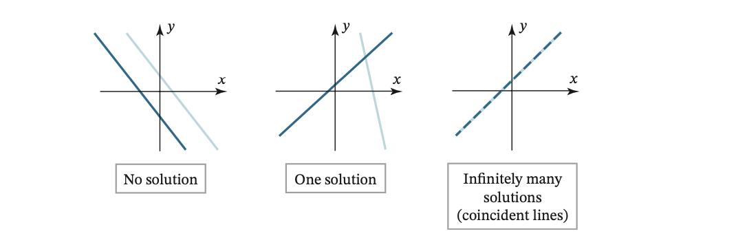
If a system has at least one solution it is called consistent, otherwise, inconsistent, thus a consistent linear system has either one solution or infinitely many solutions, and this extends to systems of equations in three unknowns, for example, the following system, the graphs of which are planes:
While these planes can relate to each other in six different ways now, the solution(s) of the system are still restricted to the three types of possibilities:

Augmented Matrices & Elementary Row Operations
The higher the number of equations in a system, the higher the complexity of the algebra required to find a solution: this can be made more simple by removing the 's, the variables, and the 's.
This allows us to write the system , as so:
This is the augmented matrix for the system.
The basic method for solving a system is to apply algebraic operations to the system that preserve the solution set, to produce increasingly simple systems, until it can be determined if the system is consistent.
The algebraic operations are:
Multiplying each term of an equation by a constant.
Interchanging two equations.
Multiplying each term of an equation by a constant and adding it to another equation.
Due to the relationship between rows of a matrix and equations in a system, these operations are easily applied to matrices, where equations become the rows.
Exercise Set 1.1
1. For each equation, determine whether the equation is linear in and :
a.) .
Linear in all three. The third term, was tricky, as linear equations do not involve roots of variables, so seeing a radical confused me, but it turns out, in this case, is a constant by which is multiplied, and thus is valid.
b.)
Not linear in all three. The terms and are linear, but is a product of variables, which is a violation of the definition of a linear equation.
c.)
Linear in all three, no products, roots of variables, or powers beyond the first.
Also, this can be re-written as , which shows the linearity more clearly, using the law of inverses.
d.)
Not linear in all three, as the term is raised to the second power, and violates the definition of a linear equation.
e.)
Not linear in all three.
f.)
Not linear in all three.
2. For each equation, determine whether the equation is linear in and :
a.)
Linear in both.
b.)
Not linear in both, due to exponentiation of the first variable in the first term and the square root of the second variable in the second term.
c.)
Linear in both. The first term is a bit dense but is a constant by which the variable is multiplied- the variable itself is consistent with definitions of linear equations.
d.)
Not linear in both as the cos(x) is a trigonometric function applied to the first variable which is a violation of the definition of linear equations.
e.)
Not linear in both, products of variables aren't valid.
f.) .
Linear in both, also can be rewritten as .
3. Using the notation of formula 7, write down a general linear system of:
a.) two equations in two unknowns:
b.) three equations in three unknowns
c.) two equations in four unknowns
4. Write down the augmented matrix for each system in exercise 3.
a.)
b.)
c.)
5-6.) In exercises 5-6, find a system of linear equations in the unknowns that corresponds to the given augmented matrix.
a1.)
b1.)
a2.)
b2.)
7-8. Find the augmented matrix for the linear system.
a1.)
b1.)
c1.)