Physics Lournal
Powered by 🌱Roam GardenQuick Calculus
Functions and Graphs
One of the most important structures in Calculus is the the function: it is an association between the elements of two sets.
The set of input values to a function is called the domain of the function.
Usually, we use to denote an element of the domain, which is referred to as the independent variable.
If (an element of the codomain of the function) represents an element that is associated with , then is referred to as the independent variable.
Dependent variables are elements of the codomain, and independent variables are elements of the domain. The range of the function are the elements of codomain that are acceptable according to the rules defined by the function.
For example, if represents a time of day, and is a temperature, is the independent variable, and is the dependent variable.
Generally, specifying a function entails listing the details of the association between two elements. Another method is to present a rule for isolation the dependent variables in terms of the independent variable, which is often an equation:
.
Typically, the allowed values are listed as well.
Unless stated otherwise, the independent variable can be any real number, for which the dependent variable is also a real number.
Functions are represented by , and the dependent variable associated with the independent variable by the function , is , written in its entirety ass .
This means we can rewrite the above value , like so:
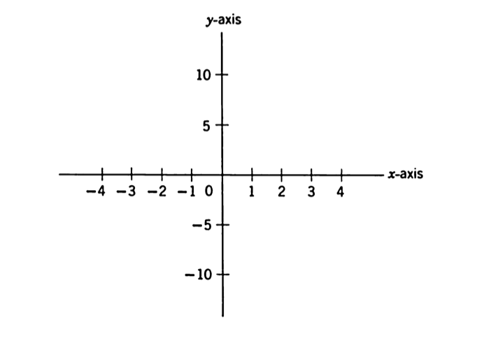
One of the common techniques for representing a function is a graph, which is constructed of intersecting coordinate axes, where the intersection is valued zero for all axes, referred to as the origin. The vertical coordinate axis is named the y-axis, and the horizontal axis is named the x-axis.
 Note: the scale of the x and y axes do not have to be the same, and neither do the units.
We can use this to represent a pair of values like so: if we let be the independent variable , and be the dependent variable , then we see .
We can extend a line parallel to the y-axis, at distance from that axis, and extend another line parallel to the x-axis, at distance , and the point at which these lines intersect is designated by the pair of values for .
The number is the x-coordinate of , and the number is the y-coordinate of . In more technical language, the value is referred to as the abscissa, and the value is referred to as the ordinate.
The simplest way of plotting the graph of some function , is to calculate a table of values of , and the corresponding values of .
There are also special kinds of functions, which have dependent variables which do not fluctuate with independent variables, referred to as constant functions, such as this function which assigns a fixed number to every variable , meaning .
Another simple function is the absolute value function, which is defined by a value surrounded by a pair of bars: , which determines the value of a number regardless of its sign.
$$|x| = \begin{cases} x\; \text{if}\; x \geqslant \; 0, \
-x\; \text{if}\; x \lt 0 \end{cases} $$
Linear and Quadratic Functions
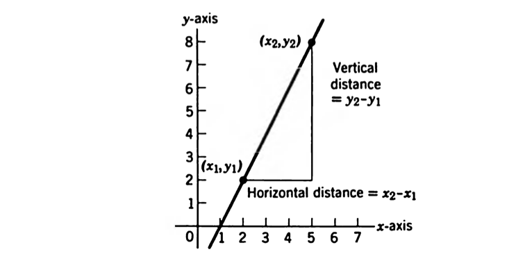
Linear functions are equations of the form , and it is called so because graphing the values produces a line.
A graph of a typical linear function looks like the following:

Should the and scale be the same, the slope is the ratio of vertical distance to horizontal distance as we travel from one point on the line to another, and the slope is the same regardless of which pair of points you choose.

If the line is vertical, the slope is infinite.
If the scales are not the same, the slope doesn't change, but it must be described with the appropriate scale: the following two figures may look the same, but have different slopes:
 Slopes: , respectively.