Mathematics Science Physics

Link

Linear Algebra is the lingua franca of Quantum Computation.

Understanding of the basic mathematical concepts that it contains, are necessary to build and analyze the structures of quantum computation.

Vectors and Vector spaces.

At the outset, the fundamental quantity in quantum computation is the vector.

A vector $| v \rangle$ , is defined as elements of a set known as a Vector Space.

Example of a vector quantity:
Velocity: The rate at which a position is changing over time.
.

You can conceptualize a vector geometrically as something having magnitude and direction, for instance a vector with x and y components $\footnotesize \begin{pmatrix}3 \ 5 \end{pmatrix}$ , more generally $\footnotesize \begin{pmatrix}x\ y \end{pmatrix}$

Within quantum computing, we often work with state vectors, vectors that represent a specific point in space that corresponds to some state in a quantum system, which can be visualized via a bloch sphere:

This particular vector state corresponds to an even superposition between $| 0 \rangle$ and $| 1 \rangle$ .

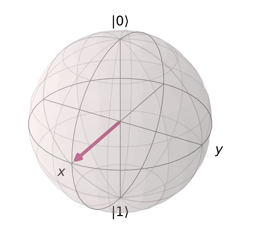
Vectors can rotate (around the center) to any point on the surface of the sphere, and each point represents a unique state of some quantum system.

In order to completely define vectors, we must define vector space:

A vector space $V$ over a field $F$ , is a set of vectors, where two conditions hold:

Vector addition of two vectors $| a \rangle,\; |b \rangle \in V$ , will yield a third vector $| a \rangle,\; | b \rangle = | c \rangle$ , which is also in $V$ .

Scalar multiplication between $| a \rangle \in V$ and some $n \in F$ , written $n|a \rangle$ , is also contained in $V$ .

A field, in this context, can be thought of as some set of numbers, with the property that if $a,b \in F$ , then aand b can be added, subtracted, multiplied and divided.

To clarify this, we will do an example, demonstrating the set $\R^{2},$ over a field $\R$ is a vector space, meaning:

$\footnotesize \begin{pmatrix} x_{1}\ y_{1} \end{pmatrix} + \begin{pmatrix} x_{2}\ y_{2} \end{pmatrix} = \begin{pmatrix} x_{1} + y_{2} \ x_{2} + y_{2} \end{pmatrix}$ , is also contained in $\R^{2}$ .

This is true because the sum of two real numbers is also a real number, meaning both new vector components are real numbers, and so they must reside in $\R^{2}$ .

Sidenote: A field in $\R^{2}$ is written as $\R$ , because it's a plane.

We also state that:

$n|v \rangle = \begin{pmatrix} nx \ ny \end{pmatrix} \in V\;, \forall n \in \R$

Scaling a vector.

Matrices and Matrix operations.

Another fundamental structure is that of the matrix, which can transform vectors into other vectors: $|v \rangle \rightarrow |v' \rangle = M|v \rangle$ .

Matrices can be represented as arrays of numbers:

$M = \begin{pmatrix} 1 & -2 & 3\ 1 & 5i & 0\ 1 + i & 7 & -4 \end{pmatrix}$

A matrix can be applied to vectors, via matrix multiplication.

Generally, we take the first row of the first matrix, and multiply each element by its corresponding element in the column of the second matrix.

The sum of these elements, is the first element, in the first row of the new matrix. To fill the rest of the row, we take the first row of the first matrix by the rest of the columns of the second matrix exhaustively.

Then, we take the second row of the first matrix, and repeat the process for each column of the second matrix, until we've used all rows of the first matrix.

$\footnotesize \begin{pmatrix} 2 & 0\ 5 & 1 \end{pmatrix} \begin{pmatrix} 3 & 1\ 2 & 1 \end{pmatrix}=$ $\footnotesize \begin{pmatrix} (2)(-3) + (0) + 2 & (2)(1) + (0)(1)\ (5)(-3) + (-1)(2) & (5)(1) + (-1)(1) \end{pmatrix}=$

$\footnotesize \begin{pmatrix} -6 & 2\ -17 & 4 \end{pmatrix}$

In order to carry out quantum computations, we take a quantum state vector, and manipulate it by applying a matrix to it. A vector is simply a matrix that only has one column. To carry out this multiplication, we carry out the above procedure. We manipulate qubits by applying sequences of quantum gates, which can be expressed as matrices of elements that alter the states of qubits, such as the Pauli-X gate:

$\sigma_{x} = \begin{pmatrix} 0 & 1\ 1 & 0\end{pmatrix}$ .

The Pauli-X gate manipulates single qubits, and is the quantum equivalent of the not gate in classical computation, and is represented by the Pauli-X matrix: $\footnotesize \begin{bmatrix} 0 & 1\ 1 & 0 \end{bmatrix}$ .

It flips the computational basis states, which are written as column vectors:

$| 0\rangle=\begin{pmatrix} 1\ 0\end{pmatrix}\; |1\rangle = \begin{pmatrix} 0\ 1 \end{pmatrix}$

When we apply the Pauli-X matrix to the vectors:

$\footnotesize \sigma_{x}|0\rangle = \begin{pmatrix} 0 & 1\ 1 & 0 \end{pmatrix} \begin{pmatrix} 1 & 0 \end{pmatrix} = \begin{pmatrix} (0)(1) + (1)(0)\ (1)(1) + (0)(0) \end{pmatrix} = \begin{pmatrix} 0\ 1 \end{pmatrix} = |1\rangle$

$\footnotesize \sigma_{x}|1\rangle = \begin{pmatrix} 0 & 1\ 1 & 0 \end{pmatrix} \begin{pmatrix} 0 & 1 \end{pmatrix} = \begin{pmatrix} (0)(0) + (1)(1)\ (1)(0) + (0)(1) \end{pmatrix} = \begin{pmatrix} 0\ 1 \end{pmatrix} = |0\rangle$

A Hermitian matrix is a matrix is that is equivalent to its Conjugate Transpose denoted $\dagger$ , which means if you flip the signs of the imaginary components of the matrix, and then reflect these components over the top left diagonal, the resulting matrix will be the one you started with:

$\sigma_{y} = \begin{pmatrix} 0 & -i\ i & 0 \end{pmatrix} \implies \sigma_{y}^{\dagger} = \begin{pmatrix} 0 & -(i)\ -(-i) & 0 \end{pmatrix}\ = \begin{pmatrix} 0 & -i\ i & 0 \end{pmatrix} = \sigma_{y}$

A Unitary matrix is similar, in that the inverse matrix is equal to the conjugate transpose.

The inverse of some matrix A, denoted $A^{-1}$ , is a matrix such that: $A^{-1}A = AA^{-1} = []$ , where $[]$ is the identity matrix.

The identity matrix has 1's along the top left diagonal, and 0's elsewhere.

When matrices grow beyond 2x2, calculating inverses is tedious, and is usually left to computers, but for a 2x2 matrix, we define the inverse as:

$A = \begin{pmatrix} a & b\ c & d \end{pmatrix} \implies A^{-1} = \frac{d}{det\;A} \begin{pmatrix} d & -b\ -c & a \end{pmatrix}$ , where $det\; A$ is the determinant of the matrix. In this 2x2 case, $det\; A = ad - bc$ .

Calculating inverses is rarely important, since Unitary matrices inverses are given by the conjugate transpote.

The Pauli-Y matrix, for instance, is Hermitian, and unitary, meaning it is it's own inverse:

$\sigma_{y} = \begin{pmatrix} 0 & -i\ i & 0 \end{pmatrix} \sigma_{y}^{\dagger} = \begin{pmatrix} 0 & -i\ i & 0 \end{pmatrix} \implies \sigma_{y}^{\dagger}\sigma_{y} = \begin{pmatrix} (0)(0) + (-i)(i) & (0)(i) + (-i)(0)\ (i)(0) + (0)(i) & (i)(-i) + (0)(0) \end{pmatrix} = \begin{pmatrix} 1 & 0\ 0 & 1 \end{pmatrix} = []$

The basic idea is that evolving a quantum state via the application of a unitary matrix preserve the magnitude of the quantum state.

Spanning Sets, Linear Dependence and Bases

Here, we will take a look at the construction of vector spaces: Consider some vector space $V$ . We say that some set of vectors of $S$ spans some subset of the vector space (subspace), expressed by $V_{s} \sub V$ , if we can write any vector in the subspace, as a Linear Combination of the other vectors in the space.

This subset notation indicates that there are elements of $V$ that are not within $V_{s}$ .

A linear combination of some set of vectors, in a space over a field $F$ , is arbitrarily defined as the sum of said vectors, which will also be a vector:

$|v\rangle = f_{1}|v_{1}\rangle + f_{2}|v_{2}\rangle + ... + f_{n}|v_{n} = \sum\limits_{i} f_{i}|v_{i}\rangle$ , where each $f_{i}$ is some element of $F$ . If we have a set of vectors spanning some space, any other vector in that space, can be described by those other vectors.

A set of vectors $|v_{1}\rangle,...|v_{n}\rangle$ is linearly dependent if there exist corresponding coefficients for each vector $b_{i} \in F$ , such that:

$b_{1}|v_{1}\rangle + b_{2}|v_{2}\rangle,...b_{n}|v_{n}\rangle = \sum\limits_{i}b_{i}|v_{i}\rangle = 0$ , where at least one of the $b_{i}$ coefficients is non-zero. For example if we have $|v_{1}\rangle, ..., |v_{n}\rangle$ , and some coefficients $|b_1\rangle, ..., |b_n\rangle$ , such that the linear combination is 0.

Since there's a vector with a non-zero coefficient (a non-zero scalar applied to the basis vector), we choose that term, $b_{a}|v_{a}\rangle$ :

$\sum\limits_{i} \ b_i |v_i\rangle \ = \ b_a |v_a\rangle \ + \ \displaystyle\sum\limits_{i, \ i \ \neq \ a} \ b_i |v_i\rangle \ = \ 0 \ \Rightarrow \ |v_a\rangle \ = \ - \displaystyle\sum_{i, \ i \ \neq \ a} \ \frac{b_i}{b_a} |v_i\rangle \ = \ \displaystyle\sum\limits_{i, \ i \ \neq \ a} \ c_i |v_i\rangle$

If $b_{a}$ is the only non-zero coefficient, then $|v_{a}\rangle$ has been written as the null vector, meaning the set is linearly dependent. Otherwise, $v_{a}$ would be described as some element of the combination of non-zero vectors above. To prove the converse, we assume some vector $|v_{a}\rangle$ in the subspace $|v_{1}\rangle,...|v_{n}\rangle$ that can be written as a linear combination of other vectors:

$|v_{a}\rangle = \sum\limits_{s}{b_{s}|v_{s}\rangle}$ , where $s$ is an index that spans the a subset of the subspace.

From this we get: $\tiny |v_{a}\rangle = \sum\limits_{s}{b_{s}|v_{s}\rangle} = |v_{a}\rangle - (b_{1}|v_{s_{1}}\rangle + ... + b_{r}|v_{s_{r}}) = 0$

Essentially, for all vectors that are not included in the subset, we set their coefficients, indexed by q, to 0, thus:

If we have some vectors, $\vec{v_{1}},\vec{v_{2}}, \vec{v_{3}}$ , with the following respective components: $\footnotesize \begin{bmatrix} 1\ 2\ 3 \end{bmatrix}$ , $\footnotesize\begin{bmatrix} 3\ 5\ 1 \end{bmatrix}$ , $\footnotesize \begin{bmatrix} 0\ 0\ 8 \end{bmatrix}$ , we can write $|a\rangle$ as a combination of the components of $\vec{v_{1}},\vec{v_{2}}, \vec{v_{3}}$ like so: $\begin{bmatrix} 3\ 6\ 9 \end{bmatrix} =$ $(3)\begin{bmatrix} 1\ 2\ 3 \end{bmatrix}$ , $(0)\begin{bmatrix} 3\ 5\ 1 \end{bmatrix}$ , $(0)\begin{bmatrix} 0\ 0\ 8 \end{bmatrix}$

$\footnotesize |v_a\rangle \ - \ (b_1|v_{s_1}\rangle \ + \ ... \ + \ b_r|v_{s_r}\rangle) \ + \ (0)(|v_{q_1}\rangle \ + \ ... \ + \ |v_{q_t}\rangle) \ = \ 0$ , which is a linear combination of all of the elements of the subspace.

We can consider a basic example of this process, considering the set of two vectors that live in $\R^{2}$ , $\footnotesize |a\rangle = \begin{pmatrix} 1\ 0 \end{pmatrix}$ and $\footnotesize |b\rangle = \begin{pmatrix} 2\ 0 \end{pmatrix}.$ If we choose the field over our vector space to be $\R$ , we can create a linear combination of these vectors: $2|a\rangle - |b\rangle = 0$ .

A set of vectors can be considered a linearly independent spanning set. In this context, the basis of some vector space is the minimal possible set that spans the entire space, where the cardinality of the basis set is considered the dimension of the vector space.

Bases and spanning sets are important, because the allow us to shrink vector spaces down, and speak about them as the combination of a smaller number of vectors, from which we can draw conclusions that we can generalize to the entire space, because every vector in the space is just a linear combination of basis vectors (and some scalars).

We often counter the bases of $|0\rangle, |1\rangle$ , which can be used to be describe any other qubit state via linear combinations: $\frac {|0\rangle + |1\rangle}{\sqrt 2}$ , representing an even superposition between the two possible states.

Hilbert Spaces, Orthonormality, Inner Products

One of the premiere mathematical structures of Quantum Mechanics is the Hilbert Space. Here, we can think of Hilbert spaces as a state space in which all vectors representing quantum states exist. The difference between these spaces, and typical vector spaces, is that Hilbert space comes equipped with an inner product, an operation that can be performed on two vectors, that returns a scalar.

The scalar quantity returned from this operation represents the degree to which the first vector lies along the second vector. From this value, the probabilities of measurement in different quantum states can be calculated.

For two vectors a and b, in a Hilbert space, the inner product is described as $\langle a |b\rangle$ , where a and b are conjugate transposes of their original values, giving us:

$\footnotesize \langle a | b \rangle \ = \ \begin{pmatrix} a_1^{} & a_2^{} & ... & a_n^{} \end{pmatrix} \begin{pmatrix} b_1 \ b_2 \ . \ . \ . \ b_n \end{pmatrix} \ = \ a_1^{} b_1 \ + \ a_2^{} b_2 \ + \ ... \ + \ a_n^{} b_n$ , where * denotes the complex conjugate of some vector.

One of the most important conditions for these spaces, is that the inner product of some vector with itself is equal to one: $\langle \psi | \psi \rangle = 1$ . This is the normalization condition expressed mathematically, which states the length of the vector squared (the components squared and summed), is equal to one. The physical significance is that the length of a vector in a particular direction is representative of the probability amplitude of the quantum system, with regard to the measurement of some quantum state.

Returning to the Bloch sphere:

The surface of this sphere is a valid Hilbert Space, along with the inner product between qubit states. A final note on Hilbert spaces is that they relate to Unitary matrices, which preserve inner product, meaning you can transform a vector under a series of unitary matrices without breaking the normalization condition that the inner product of two vectors must equate to one:

$\footnotesize \langle \psi | \psi \rangle \ = \ 1 \ \Rightarrow \ |\psi\rangle \ \rightarrow \ U |\psi\rangle \ = \ |\psi'\rangle \ \Rightarrow \ \langle \psi' | \psi' \rangle \ = \ (U |\psi\rangle)^{\dagger} U|\psi\rangle \ = \ \langle \psi | U^{\dagger} U |\psi\rangle \ = \ \langle \psi | \psi \rangle \ = \ 1$

This means Unitary evolution of quantum systems sends quantum states to other valid quantum states- for a single qubit Hilbert space, represented by the Bloch sphere, unitary transformations correspond to vector rotations to different points on the sphere, without altering the length of the vector.

Outer Products and Tensor Products

Qiskit: Intro to Linear Algebra

Mathematics Science Physics

Link

Linear Algebra is the lingua franca of Quantum Computation.

Understanding of the basic mathematical concepts that it contains, are necessary to build and analyze the structures of quantum computation.

Vectors and Vector spaces.

At the outset, the fundamental quantity in quantum computation is the vector.

A vector ∣v⟩| v \rangle∣v⟩, is defined as elements of a set known as a Vector Space.

Example of a vector quantity: Velocity: The rate at which a position is changing over time..

Velocity: The rate at which a position is changing over time.

You can conceptualize a vector geometrically as something having magnitude and direction, for instance a vector with x and y components (3 5)\footnotesize \begin{pmatrix}3 \ 5 \end{pmatrix}(3 5​), more generally (x y)\footnotesize \begin{pmatrix}x\ y \end{pmatrix}(x y​)

Within quantum computing, we often work with state vectors, vectors that represent a specific point in space that corresponds to some state in a quantum system, which can be visualized via a bloch sphere:

This particular vector state corresponds to an even superposition between ∣0⟩| 0 \rangle∣0⟩ and ∣1⟩| 1 \rangle∣1⟩.

Vectors can rotate (around the center) to any point on the surface of the sphere, and each point represents a unique state of some quantum system.

In order to completely define vectors, we must define vector space:

A vector space VVV over a field FFF, is a set of vectors, where two conditions hold:

Vector addition of two vectors ∣a⟩, ∣b⟩∈V| a \rangle,\; |b \rangle \in V∣a⟩,∣b⟩∈V, will yield a third vector ∣a⟩, ∣b⟩=∣c⟩| a \rangle,\; | b \rangle = | c \rangle∣a⟩,∣b⟩=∣c⟩, which is also in VVV.

Scalar multiplication between ∣a⟩∈V| a \rangle \in V∣a⟩∈V and some n∈Fn \in Fn∈F, written n∣a⟩n|a \ranglen∣a⟩, is also contained in VVV.

A field, in this context, can be thought of as some set of numbers, with the property that if a,b∈Fa,b \in Fa,b∈F, then aand b can be added, subtracted, multiplied and divided.

To clarify this, we will do an example, demonstrating the set R2,\R^{2},R2, over a field R\RR is a vector space, meaning:

(x1 y1)+(x2 y2)=(x1+y2 x2+y2)\footnotesize \begin{pmatrix} x_{1}\ y_{1} \end{pmatrix} + \begin{pmatrix} x_{2}\ y_{2} \end{pmatrix} = \begin{pmatrix} x_{1} + y_{2} \ x_{2} + y_{2} \end{pmatrix}(x1​ y1​​)+(x2​ y2​​)=(x1​+y2​ x2​+y2​​), is also contained in R2\R^{2}R2.

This is true because the sum of two real numbers is also a real number, meaning both new vector components are real numbers, and so they must reside in R2\R^{2}R2.

Sidenote: A field in R2\R^{2}R2 is written as R\RR, because it's a plane.